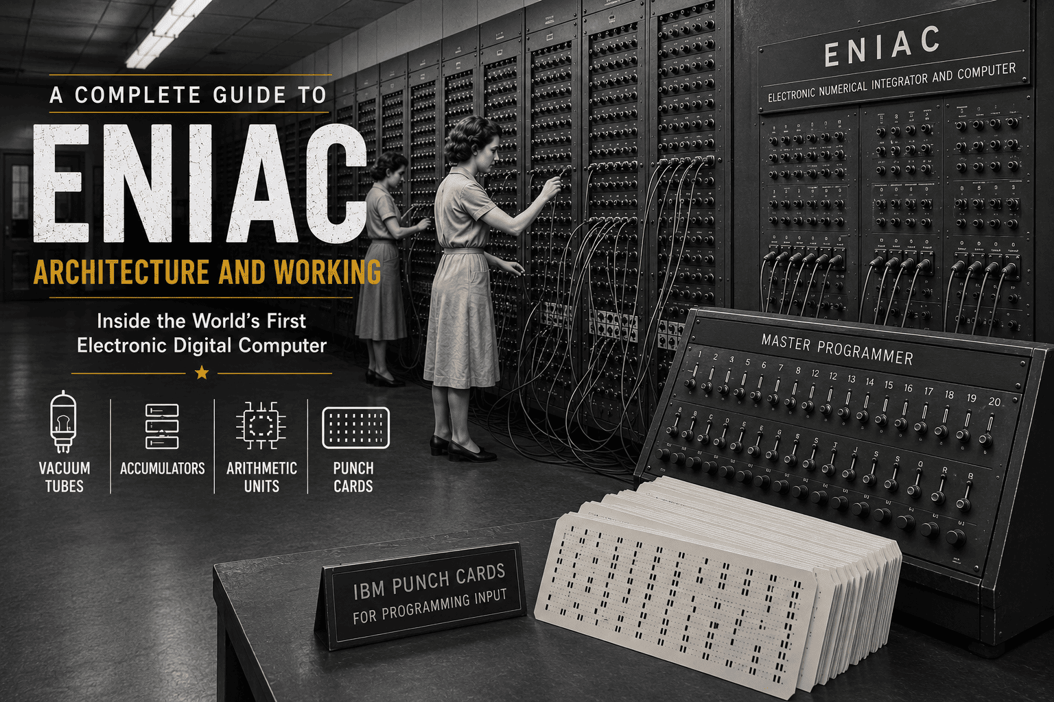
Understanding ENIAC Architecture and Working is one of the best ways to learn how the ENIAC computer, the world’s first general-purpose electronic digital computer, revolutionised modern computing. While today’s computers perform billions of calculations every second using tiny microprocessors, ENIAC achieved remarkable computational speeds using thousands of vacuum tubes, electronic circuits, and manually configured hardware. Exploring how this pioneering machine worked provides valuable insight into the evolution of computer architecture.

If you’re new to the ENIAC computer, we recommend reading our Beginner’s Guide to ENIAC first. It explains what ENIAC is, why it was developed, who built it, and why it remains one of the most significant milestones in ENIAC history. Once you’re familiar with those fundamentals, this tutorial will help you understand how the machine actually operated internally.

Unlike modern computers, ENIAC had no operating system, no programming language, and no stored programs. Engineers programmed the machine by connecting patch cables, setting switches, and configuring plugboards before entering numerical data through IBM punch cards. Although this process was time-consuming, it allowed ENIAC to solve complex mathematical problems much faster than any previous machine.

In this tutorial, you’ll explore the complete ENIAC Architecture and Working, including its vacuum tubes, accumulators, Master Programmer, function tables, arithmetic units, data flow, and programming model. By the end, you’ll understand not only how the ENIAC computer worked, but also why its architecture laid the foundation for the development of modern digital computers.

Why Study ENIAC Architecture?

At first, studying a computer built during the 1940s may not seem particularly useful. After all, modern computers are millions of times faster, dramatically smaller, and far easier to use.

So why do universities around the world still teach ENIAC?

The answer is simple.

ENIAC represents the beginning of practical electronic computing. Before ENIAC, most calculations were performed manually or with mechanical machines that relied on gears, shafts, and rotating wheels. These machines were useful but painfully slow when solving large mathematical problems.

ENIAC changed that forever.

For the first time, engineers proved that an entirely electronic machine could solve complicated calculations at speeds that had never been achieved before. Although today’s computers use microprocessors instead of vacuum tubes, many of the fundamental ideas introduced during ENIAC’s development continue to appear in modern computer architecture.

Studying ENIAC helps you understand concepts such as:

Electronic computation
Digital logic
Computer architecture
Data processing
Parallel processing
Hardware-based programming
Evolution of modern computers

More importantly, ENIAC teaches an important lesson:

Modern computers did not appear overnight. They evolved through decades of engineering innovations, and ENIAC was one of the most significant milestones in that journey.

Before We Explore the Architecture…

Let’s begin with a simple example. Imagine you need to calculate:

248 × 136

Today, you would probably open the Calculator application on your phone or laptop. Within a fraction of a second, the answer appears on the screen.

Now imagine performing exactly the same calculation on the ENIAC computer.

You couldn’t simply type the numbers.

There was no keyboard.

There was no display.

There was no software.

Instead, a team of trained operators first had to decide which electronic units would perform each part of the calculation. They manually connected patch cables between different panels, adjusted hundreds of switches, configured arithmetic units, and verified that every electrical connection represented the correct sequence of operations.

Only after this physical setup was complete could numerical data be supplied using IBM punch cards.

Although the preparation could take several hours – or even days for complex problems – the actual calculation often finished in only a few seconds.

This difference is important.

Modern computers spend almost no time preparing a program because software is already stored in memory.

ENIAC spent most of its time preparing the program rather than executing it. Understanding this single difference makes the rest of ENIAC’s architecture much easier to understand.

The Philosophy Behind ENIAC

When people first see photographs of ENIAC, they often ask one question:

“Where is the CPU?”

The surprising answer is:

ENIAC didn’t have one.

This is one of the biggest differences between the ENIAC computer and every modern computer you use today.

A modern computer contains a Central Processing Unit (CPU) that performs calculations, controls memory, and coordinates every operation within the system.

ENIAC followed a completely different philosophy.

Instead of relying on one processor to perform every task, ENIAC divided the workload among many specialised electronic units.

Think of a modern restaurant.

Rather than asking one person to prepare every meal, different employees perform different jobs. One chef cooks the food, another prepares desserts, someone else manages orders, and another person serves customers. Each worker specialises in one task, allowing the restaurant to operate more efficiently.

ENIAC worked in a similar way.

Instead of building one enormous electronic brain, its designers created multiple specialised units.

Some units stored numbers. Others performed multiplication. Another handled division. Some coordinated the order of calculations. Others supplied constant numerical values.

By allowing these specialised units to work together, ENIAC could perform several operations simultaneously – a remarkable achievement during the 1940s.

This modular design is one of the reasons ENIAC is recognised as the world’s first successful general-purpose electronic digital computer.

Overall Architecture of the ENIAC Computer

Unlike today’s computers, which place billions of transistors onto a processor smaller than your fingertip, the ENIAC computer occupied an entire room.

It weighed approximately 30 tons, covered nearly 1,800 square feet (167 square metres) of floor space, and consumed around 150 kilowatts of electrical power. The machine consisted of forty large panels arranged in a U-shaped layout, allowing engineers to access both the front and rear for maintenance and programming.

Behind these metal panels were thousands of electronic components working together as one integrated system.

Some of the most important hardware included:

Component	Purpose
20 Accumulators	Stored numbers and performed addition or subtraction
High-Speed Multiplier	Performed multiplication operations
Divider/Square Root Unit	Calculated division and square roots
Function Tables	Stored frequently used numerical constants
Master Programmer	Controlled the sequence of operations
Cycling Unit	Generated timing pulses that synchronised the machine
Initiating Unit	Started, stopped, and reset computations
Constant Transmitter	Supplied predefined numerical constants
IBM Card Reader	Read numerical input from punch cards
IBM Card Punch	Recorded results onto new punch cards

Each unit performed a specific responsibility, yet none of them worked alone.

Instead, electrical pulses continuously travelled between these units through thousands of wires and manually connected patch cables.

Rather than executing software instructions stored in memory, ENIAC executed electrical pathways that had been physically created by its operators.

In other words, the program wasn’t stored inside ENIAC.

The program was the wiring itself.

That single idea makes ENIAC fundamentally different from every modern computer.

How Was ENIAC Programmed?

One of the biggest misconceptions about ENIAC is that operators simply inserted a punch card containing a program, much like loading software into a modern computer.

That never happened.

In reality, programming ENIAC resembled building an electrical circuit rather than writing computer code.

When engineers wanted ENIAC to solve a new mathematical problem, they first studied the calculation and divided it into smaller operations such as addition, subtraction, multiplication, comparison, or data transfer.

Next, they physically connected different electronic units using thick patch cables.

Thousands of switches had to be positioned correctly.

Plugboards needed to be configured.

Function tables had to be loaded with appropriate numerical constants.

Only after every electrical connection had been carefully verified was the machine ready to receive numerical input through IBM punch cards.

Changing the program often required reconnecting hundreds of cables, meaning that a new calculation could take hours – or even days – to prepare.

Although this seems incredibly inefficient today, it represented a revolutionary breakthrough during the 1940s because the same hardware could now solve many different kinds of problems simply by changing its wiring.

This flexibility distinguished ENIAC from earlier special-purpose machines and helped establish it as one of the world’s first practical general-purpose electronic digital computers.

Now that you understand why ENIAC was designed this way, the next question naturally follows:

How did thousands of vacuum tubes actually perform calculations using nothing more than electrical signals?

To answer that, we’ll step inside the heart of ENIAC and explore the electronic technology that made this remarkable machine possible. We’ll begin with vacuum tubes, the fundamental building blocks of the ENIAC Architecture and Working, before moving on to accumulators, arithmetic units, function tables, and the complete data-processing workflow.

Vacuum Tubes: The Electronic Heart of ENIAC

If the accumulators were the “workers” of the ENIAC computer, then the vacuum tubes were its beating heart.

Every calculation performed by ENIAC—from adding two numbers to solving complex ballistic equations—ultimately depended on these electronic devices. Without vacuum tubes, ENIAC would never have become the world’s first successful general-purpose electronic digital computer.

To appreciate their importance, let’s first understand what a vacuum tube actually is.

What Is a Vacuum Tube?

A vacuum tube, also known as a thermionic valve, is an electronic device that controls the flow of electric current inside a sealed glass tube from which most of the air has been removed. Long before the invention of transistors and integrated circuits, vacuum tubes were widely used to amplify electrical signals and act as electronic switches.

Think of a vacuum tube as an electronic tap connected to a water pipe.

When the tap is closed, water cannot flow.
When the tap is opened, water flows freely.

A vacuum tube performs a similar function, except that instead of controlling water, it controls the flow of electrons. By rapidly allowing or stopping the movement of electrons, vacuum tubes create electrical pulses that represent digital information.

In modern computers, this job is performed by tiny transistors. However, during the 1940s, vacuum tubes were the fastest electronic switching devices available.

Why Did ENIAC Need So Many Vacuum Tubes?

One of the most fascinating facts about the ENIAC computer is the enormous number of vacuum tubes it contained.

ENIAC used approximately 17,468 vacuum tubes – a figure commonly rounded to 18,000 in many textbooks. These tubes were distributed across the machine’s various functional units, including the accumulators, arithmetic circuits, and control systems.

You might wonder why so many tubes were necessary.

The answer lies in how ENIAC processed information.

Unlike modern processors, where billions of transistors are integrated onto a single silicon chip, ENIAC’s electronic circuits were built using individual components. Each logical operation, storage function, or arithmetic process required numerous vacuum tubes working together. Even a simple addition involved thousands of electronic switching operations occurring almost simultaneously.

As a result, a single calculation activated a vast network of tubes throughout the machine.

Although this design occupied an entire room, it enabled ENIAC to perform calculations at unprecedented speeds for its era.

How Did Vacuum Tubes Perform Calculations?

At first glance, it seems impossible that glass tubes could solve mathematical problems.

The key is understanding that ENIAC never “thought” about numbers the way humans do.

Instead, it processed electrical pulses.

Imagine a light switch. When the switch is ON, electricity flows. When the switch is OFF, electricity stops.

Vacuum tubes operated on a similar principle. They rapidly switched electrical signals on and off thousands of times every second. By combining thousands of these switching operations, ENIAC created electronic circuits capable of performing arithmetic calculations.

For example, when ENIAC needed to add two numbers, electrical pulses representing each digit travelled through specially designed circuits. Vacuum tubes controlled the movement of these pulses, ensuring they reached the correct accumulators and arithmetic units in the proper sequence.

Although today’s computers use binary digits (0s and 1s), ENIAC primarily processed decimal digits, making its internal design significantly different from modern processors.

Did Vacuum Tubes Store Information?

This is a common misconception.

Vacuum tubes themselves did not store numbers.

Instead, they acted as electronic switches that controlled the movement of electrical signals throughout the machine. The actual temporary storage of numbers occurred inside units called accumulators, which we’ll study shortly.

You can think of the relationship like this:

Vacuum tubes moved electrical signals.
Accumulators held numerical values.
Control units determined where those values should go next.

Each component had a unique responsibility, and together they formed one coordinated computing system.

The Biggest Challenge: Heat and Reliability

Although vacuum tubes transformed electronic computing, they also introduced significant engineering challenges.

Each tube generated heat while operating. Now imagine nearly 18,000 of them working continuously inside one machine. The result was enormous heat generation.

To keep ENIAC functioning reliably, powerful ventilation systems circulated air throughout the machine. Even with cooling, individual tubes occasionally failed due to the high operating temperatures.

Contrary to popular myths, ENIAC did not experience tube failures every few minutes. As engineers improved maintenance procedures and left the machine powered on continuously, reliability increased considerably. By the late stages of its operation, ENIAC often ran for many hours before a tube required replacement.

Even so, maintaining such a large electronic system demanded constant attention from engineers and technicians.

Vacuum Tubes vs Modern Transistors

Understanding the difference between vacuum tubes and transistors helps explain why modern computers are dramatically smaller and more powerful.

Feature	Vacuum Tubes (ENIAC)	Modern Transistors
Technology	Glass electronic device	Semiconductor device
Size	Several centimetres tall	Measured in nanometres
Heat Generation	Very High	Extremely Low
Power Consumption	High	Very Low
Reliability	Limited lifespan	Highly reliable
Switching Speed	Fast for the 1940s	Billions of operations per second
Quantity	About 18,000	Billions on a single processor

Although modern transistors have replaced vacuum tubes, both perform the same fundamental task: controlling the flow of electrical signals.

In many ways, today’s processors are descendants of the electronic switching principles first demonstrated by machines like ENIAC.

Why Vacuum Tubes Changed Computing Forever

Before ENIAC, most calculating machines relied on mechanical parts such as gears, wheels, and levers. Mechanical movement limited their speed because every calculation depended on physical motion.

Vacuum tubes removed this limitation.

Since electrical signals travel much faster than mechanical components can move, ENIAC completed calculations at speeds that seemed extraordinary during the 1940s.

For example, ENIAC could perform approximately:

5,000 additions per second
357 multiplications per second
38 divisions per second

These performance figures represented a revolutionary leap over earlier electromechanical machines.

More importantly, they proved that electronic computing was not just possible—it was practical.

This breakthrough encouraged engineers around the world to develop newer and more efficient electronic computers, eventually leading to transistor-based systems, integrated circuits, microprocessors, and the powerful computers we use today.

From Electronic Signals to Numbers

So far, we’ve learned how vacuum tubes controlled the movement of electrical pulses throughout ENIAC.

However, electrical pulses alone cannot solve mathematical problems.

The machine also needed a place to store numbers temporarily, perform arithmetic operations, and pass results to other parts of the system.

That responsibility belonged to one of the most remarkable components of the ENIAC architecture – the Accumulator.

Accumulators: The Working Memory and Calculator of ENIAC

If vacuum tubes were the electronic heart of the ENIAC computer, the accumulators were its working muscles. Almost every calculation performed by ENIAC passed through one or more accumulators, making them the busiest components in the entire machine.

Modern computers separate the responsibilities of memory and processing. The RAM temporarily stores data, while the CPU performs arithmetic and logical operations. ENIAC, however, followed a different design philosophy. Each accumulator could store numbers, perform arithmetic operations, and transfer results to other parts of the machine.

For this reason, an accumulator can be thought of as a combination of a small memory unit and an arithmetic processor.

What Is an Accumulator?

An accumulator is an electronic unit designed to temporarily store numerical values while also performing arithmetic operations such as addition and subtraction.

Whenever ENIAC solved a mathematical problem, it rarely calculated the final answer in a single step. Instead, it broke the problem into many smaller calculations. After each step, the intermediate result needed to be stored somewhere before the next operation could continue.

That temporary storage location was the accumulator. Imagine solving a long mathematical equation in your notebook.

You might calculate one part of the equation, write down the answer, continue solving the next part, and then return to the previous value whenever required.

ENIAC performed a similar process electronically. Instead of writing numbers on paper, it stored them inside accumulators.

How Many Accumulators Did ENIAC Have?

The original ENIAC computer contained 20 accumulators.

Each accumulator could independently perform calculations, allowing multiple operations to occur simultaneously. This was one of the reasons ENIAC achieved extraordinary performance for the 1940s.

Rather than waiting for one calculation to finish before starting another, several accumulators could work at the same time.

This concept is similar to how modern computers execute multiple tasks in parallel, although today’s processors achieve this using entirely different technologies.

What Could an Accumulator Store?

Unlike modern computers, which represent information using binary digits (bits), ENIAC primarily worked with decimal numbers.

Each accumulator could store one signed decimal number containing up to ten digits.

For example, an accumulator could hold values such as:

3,248
145,987
9,876,543,210

It also kept track of whether the number was positive or negative, enabling ENIAC to solve a wide range of scientific and engineering problems.

Although a capacity of ten digits may seem limited today, it was more than sufficient for many of the complex calculations performed during the 1940s.

Why Did ENIAC Use Decimal Instead of Binary?

This is one of the most interesting aspects of ENIAC architecture.

Modern computers use the binary number system because electronic circuits naturally represent two states: ON and OFF.

So why didn’t ENIAC do the same? The answer lies in the historical context.

During the 1940s, engineers and mathematicians were accustomed to working with decimal numbers. Scientific tables, engineering calculations, and military computations were all expressed in decimal notation.

To make the machine easier to use and verify, ENIAC was designed to process decimal digits directly instead of converting everything into binary.

Although later computers proved that binary was more efficient, ENIAC’s decimal design simplified programming for the engineers of its time.

How Did an Accumulator Perform Addition?

Let’s see a simple example.

Suppose ENIAC needs to calculate:

245 + 175

The process would look something like this:

Step 1: The first number (245) is loaded into an accumulator.

Step 2: The second number (175) is sent to the same accumulator.

Step 3: Internal electronic circuits perform the addition digit by digit.

Step 4: The accumulator now stores the result: 420

This result can then be sent to another accumulator or directly to another arithmetic unit for further calculations.

Although this example appears simple, the same principle applies when solving much larger scientific equations involving thousands of arithmetic operations.

Carry Operations Inside an Accumulator

When adding numbers, you’ve probably encountered situations like this:

9 + 8 = 17

You write 7 in the current column and carry 1 into the next column. ENIAC had to perform exactly the same process electronically.

Each accumulator contained circuits capable of automatically generating and transferring carry values between decimal digits.

This feature was essential because scientific calculations frequently produced numbers larger than a single decimal digit. Without automatic carry handling, every addition would require additional manual processing, dramatically reducing the machine’s speed.

Accumulators Worked Together

One accumulator was rarely enough for complex calculations.

Instead, multiple accumulators cooperated throughout a program.

Imagine solving the following equation: (125+375)×(90−40)

ENIAC could divide the work among several accumulators.

For example:

Accumulator 1 stores 125.
Accumulator 2 stores 375.
Accumulator 3 calculates 125 + 375.
Accumulator 4 stores 90.
Accumulator 5 stores 40.
Accumulator 6 calculates 90 − 40.
The multiplication unit receives both intermediate results and computes the final answer.

By allowing different accumulators to work independently, ENIAC significantly reduced the overall computation time.

This was an early example of parallel processing, where multiple hardware units perform different tasks simultaneously.

Were Accumulators the Same as RAM?

Many beginners assume accumulators were simply an early version of RAM. While this comparison is understandable, it isn’t entirely accurate.

Modern Random Access Memory (RAM) is primarily designed to store data temporarily while the CPU performs calculations.

An ENIAC accumulator, on the other hand, combined two responsibilities:

It temporarily stored numerical values.
It directly performed arithmetic operations.

In other words, an accumulator behaved more like a combination of modern RAM and part of the Arithmetic Logic Unit (ALU). This unique design was one of the defining characteristics of the ENIAC computer.

Why Were Accumulators So Important?

Without accumulators, ENIAC would have been little more than a collection of electronic switches.

These units provided a place where numbers could be stored, modified, and exchanged with other components during a calculation. Because almost every operation relied on accumulators, they became the central working units of the machine.

Many historians even describe them as the “workhorses” of ENIAC because they handled the majority of arithmetic processing throughout the computation.

Understanding accumulators also helps explain why ENIAC’s architecture differed so dramatically from modern computers. Rather than relying on one powerful processor, ENIAC distributed its work across multiple specialised units, each capable of contributing to the overall calculation.

High-Speed Multiplier: How ENIAC Performed Multiplication

Addition and subtraction are the foundation of arithmetic, but scientific and engineering calculations often require multiplication as well. Calculating artillery trajectories, engineering measurements, and complex mathematical equations would have been extremely time-consuming if ENIAC relied only on repeated addition performed manually.

To solve this challenge, the ENIAC computer included a dedicated hardware component known as the High-Speed Multiplier. Instead of asking the accumulators to perform every multiplication, this specialised unit was designed specifically to multiply numbers much faster and more efficiently.

This was an important engineering decision. By assigning multiplication to a dedicated hardware unit, ENIAC could continue performing other operations in parallel, improving the machine’s overall performance.

Why Was a Separate Multiplier Necessary?

Imagine you need to calculate: 245 × 36

One possible method is repeated addition.

245 + 245 + 245 + … repeated 36 times.

Although this approach eventually produces the correct answer, it is slow and inefficient, especially when dealing with very large numbers.

Engineers designing ENIAC understood this limitation.

Instead of relying entirely on repeated addition performed by the accumulators, they created a dedicated multiplication unit capable of carrying out multiplication much more quickly.

Although the multiplier still relied on the principles of repeated addition internally, its specialised electronic circuits performed these operations automatically at extremely high speeds.

How Did the High-Speed Multiplier Work?

The High-Speed Multiplier received numbers from the accumulators.

Once both values became available, the multiplier processed them electronically and generated the product. The final result was then sent back to one or more accumulators so that additional calculations could continue.

The overall process followed these steps:

The first number was stored inside an accumulator.
The second number was stored in another accumulator.
Both values were transferred to the High-Speed Multiplier.
The multiplier performed the multiplication electronically.
The resulting product was returned to an accumulator.
The calculation continued using the new value.

Although this process appears straightforward, it represented an enormous technological achievement during the 1940s.

Example: Multiplying Two Numbers

Suppose ENIAC needs to calculate: 125 × 48

The operation would proceed as follows:

Accumulator A stores 125.
Accumulator B stores 48.
Both values are sent to the High-Speed Multiplier.
The multiplier performs the necessary arithmetic operations.
The final answer, 6,000, is returned to another accumulator.

From there, ENIAC could immediately use the result in the next stage of the program.

Notice that the accumulators did not lose their importance. Instead, they worked together with the multiplier, constantly exchanging numbers throughout the calculation.

Why Was It Called a High-Speed Multiplier?

During the 1940s, multiplication was one of the most time-consuming mathematical operations.

Mechanical calculators often required several seconds – or even longer – to complete a single multiplication.

ENIAC dramatically reduced this time.

The High-Speed Multiplier could perform approximately 357 multiplications per second, making it one of the fastest multiplication systems ever built during that era.

Although modern processors perform billions of multiplications every second, ENIAC’s performance represented a revolutionary breakthrough and demonstrated the enormous potential of electronic computing.

Working Together with the Accumulators

The High-Speed Multiplier never worked in isolation. It depended on the accumulators to supply numbers and to receive completed results.

You can think of the relationship like this:

Accumulators stored the numbers.
Multiplier performed multiplication.
Accumulators stored the new result.

This continuous exchange of data allowed ENIAC to solve complex equations much faster than earlier mechanical computers.

Divider and Square Root Unit

While multiplication is an important mathematical operation, scientific calculations also require division and square root calculations.

Instead of forcing operators to perform these calculations manually, the ENIAC computer included another dedicated hardware component called the Divider and Square Root Unit.

As its name suggests, this unit performed two different mathematical operations:

Division
Square root calculations

Including both functions in a single hardware module reduced the amount of manual work required from operators and allowed ENIAC to solve much more sophisticated engineering and military problems.

Why Were These Operations More Difficult?

Addition and subtraction are relatively simple operations because they process one digit at a time.

Division, however, is much more complicated.

To divide one number by another, the machine must repeatedly compare values, subtract intermediate results, and determine when the calculation is complete.

Finding a square root is even more challenging because it requires an iterative mathematical process rather than a straightforward arithmetic operation.

These operations involve many intermediate calculations, making them considerably slower than addition or multiplication.

How Did the Divider Work?

The Divider and Square Root Unit accepted numbers from the accumulators in much the same way as the multiplier. Once the required values were available, the unit performed a sequence of electronic operations to calculate the quotient.

The completed answer was then returned to an accumulator for further processing.

For example, if ENIAC needed to calculate: 840 ÷ 12

the process would be:

Store 840 in an accumulator.
Store 12 in another accumulator.
Transfer both numbers to the Divider.
Perform the division electronically.
Return the answer (70) to an accumulator.

From there, the result could immediately participate in the next calculation.

Performance of the Divider

Division required significantly more electronic operations than multiplication.

For this reason, the Divider and Square Root Unit was slower than the High-Speed Multiplier.

On average, ENIAC could perform approximately 38 divisions per second.

Although this may appear slow by today’s standards, it was an extraordinary achievement during the mid-1940s.

Why Were Dedicated Arithmetic Units Important?

One of the reasons the ENIAC computer became so successful was that it did not force a single component to perform every mathematical operation.

Instead, engineers divided responsibilities among specialised hardware units.

Accumulators handled addition and subtraction.
The High-Speed Multiplier handled multiplication.
The Divider and Square Root Unit handled more complex mathematical operations.

This modular approach improved efficiency and allowed multiple parts of the machine to work simultaneously.

Although modern computers use a single processor containing billions of transistors, that processor still includes specialised circuits for different mathematical operations.

In many ways, ENIAC introduced the idea that different hardware components should perform different tasks – a design philosophy that continues to influence computer architecture today.

Transition to the Next Section

By now, you’ve learned how ENIAC stored numbers, performed addition, multiplication, division, and square root calculations.

However, many scientific equations repeatedly use the same numerical values, such as mathematical constants or pre-calculated coefficients. Re-entering these numbers for every calculation would have wasted valuable time.

To solve this problem, ENIAC included another ingenious component called the Function Table.

Rather than performing calculations, the Function Table stored frequently used numerical values so they could be retrieved whenever the program required them.

In the next section, we’ll explore how the Function Tables, together with the Master Programmer, coordinated complex calculations and helped transform ENIAC into one of the most powerful scientific computers of its time.

Function Tables: ENIAC’s Built-in Reference Memory

As mathematical problems become more complex, the same numbers often appear repeatedly. Scientific equations, engineering formulas, and military calculations frequently use fixed numerical values such as coefficients, conversion factors, or mathematical constants. Entering these values manually every time would not only slow down the calculation but also increase the risk of human error.

To overcome this challenge, the ENIAC computer included special units called Function Tables.

Unlike the accumulators, which temporarily stored numbers during a calculation, Function Tables stored predefined numerical values that could be reused whenever the program required them. This reduced repetitive work and made complex calculations much more efficient.

You can think of a Function Table as a reference book placed beside a student during an examination. Instead of memorising every formula, the student simply looks up the required information whenever needed. ENIAC followed a similar approach by storing important numerical values in dedicated hardware.

What Is a Function Table?

A Function Table was a hardware unit designed to store fixed decimal numbers that remained unchanged throughout a program.

These stored values could represent:

Mathematical constants
Engineering coefficients
Ballistic data
Scientific lookup values
Predefined numerical parameters

Instead of calculating or entering these numbers repeatedly, ENIAC simply retrieved them from the Function Table whenever they were required.

This approach significantly reduced programming effort and improved computational efficiency.

Why Were Function Tables Necessary?

Imagine you’re solving the following equation several hundred times: Distance=Speed×3.6

The value 3.6 never changes.

Without a Function Table, operators would need to enter 3.6 every single time the calculation was performed. Now imagine solving thousands of equations involving dozens of fixed constants. The amount of repetitive work would become enormous.

By storing these constant values inside Function Tables, ENIAC could retrieve them instantly whenever the program requested them. This simple idea greatly reduced programming complexity while also minimising the possibility of mistakes.

How Did Function Tables Work?

Unlike modern computer memory, Function Tables did not automatically store programs or user data. Instead, operators manually configured the required numerical values before running a program.

Once the machine started executing, other components could request these stored values whenever needed.

The overall process worked like this:

Operators loaded predefined constants into the Function Table.
The program reached a point where one of those constants was required.
The Function Table supplied the requested value electronically.
The value was transferred to an accumulator or arithmetic unit.
The calculation continued without requiring manual re-entry.

Although this process may seem simple today, it represented a significant innovation during the 1940s.

Real-World Example

Suppose ENIAC is calculating artillery trajectories. Each calculation requires the gravitational acceleration constant and several experimentally determined correction values.

Without Function Tables:

Operators would repeatedly enter the same constants.
Programming time would increase.
Human errors would become more likely.

With Function Tables:

The constants are entered once.
ENIAC retrieves them automatically whenever required.
Calculations proceed much faster and with greater consistency.

This capability made Function Tables especially valuable for scientific and military applications where the same numerical values appeared throughout an entire program.

Master Programmer: The Coordinator of ENIAC

One of the most misleading names in the ENIAC architecture is the Master Programmer.

When modern students hear this name, they often imagine something similar to today’s CPU or operating system.

However, neither assumption is correct. The Master Programmer was not a processor. It was not software. It did not execute programs stored in memory.

Instead, the Master Programmer acted as the central coordinator that controlled the order in which different hardware units performed their tasks.

Rather than performing calculations itself, it ensured that every component worked together in the correct sequence.

Why Did ENIAC Need a Master Programmer?

Imagine an orchestra performing a symphony.

Each musician knows how to play an instrument.

However, without a conductor, everyone might begin playing at different times, producing confusion instead of music.

The conductor does not play every instrument.

Instead, the conductor coordinates the performance.

The Master Programmer played a similar role inside ENIAC.

It did not perform arithmetic calculations.

Instead, it synchronised the activities of accumulators, multipliers, dividers, Function Tables, and other hardware units so that each operation occurred at exactly the right moment.

What Did the Master Programmer Actually Do?

The Master Programmer managed the sequence of operations by sending carefully timed electrical control pulses throughout the machine.

Its responsibilities included:

Controlling the order of calculations.
Coordinating different hardware units.
Repeating operations when necessary.
Managing loops within a program.
Synchronising complex calculations.

Without this coordination, different units might attempt to operate simultaneously when they were supposed to wait for previous calculations to finish.

The Master Programmer prevented such conflicts by ensuring that every stage of the computation followed the correct sequence.

Did the Master Programmer Read Instructions?

This is one of the biggest misconceptions surrounding the ENIAC computer.

The answer is No.

Unlike modern processors, the Master Programmer did not read software instructions from memory or punch cards.

Remember what you learned earlier. The program itself was created by manually connecting patch cables and configuring switches. Once the machine had been wired correctly, the Master Programmer simply coordinated the execution of those physical connections.

In other words, it controlled when operations occurred – not what operations were performed. The “what” had already been determined by the wiring created by the operators.

How Did It Coordinate a Program?

Let’s consider a simple sequence:

Add two numbers.
Multiply the result.
Divide the final value.
Send the answer to an output card.

The Master Programmer ensured that these operations occurred in the correct order.

First, it allowed the accumulators to complete the addition.

Only after the addition finished did it activate the High-Speed Multiplier.

Once multiplication was complete, it triggered the Divider and Square Root Unit.

Finally, it instructed the output system to record the completed result.

Without this coordination, later operations might begin before earlier calculations had finished, producing incorrect answers.

Why Is the Master Programmer Important?

Although the Master Programmer was not a CPU, it introduced one of the most important ideas in computer engineering:

Complex systems require coordination.

Modern processors include sophisticated control units that manage instruction execution, data movement, and hardware synchronisation.

While these technologies are far more advanced than ENIAC’s Master Programmer, they perform a similar fundamental role—ensuring that every part of the computer works together in the correct sequence.

For this reason, many historians consider the Master Programmer an important step in the evolution of computer control systems.

Bringing Everything Together

At this stage, you’ve explored several of the most important components of the ENIAC computer.

You now understand:

How vacuum tubes controlled electrical signals.
How accumulators stored and processed numbers.
How the High-Speed Multiplier performed multiplication.
How the Divider handled complex arithmetic.
How Function Tables supplied predefined constants.
How the Master Programmer coordinated the entire calculation.

However, one important question still remains.

How did all of these components actually work together when solving a real mathematical problem?

Understanding each individual part is valuable, but seeing the complete workflow is what truly reveals the brilliance of ENIAC Architecture and Working.

In the next section, we’ll follow a calculation from start to finish, exploring how data entered ENIAC, moved through different hardware units, and eventually became the final output.

How Did the ENIAC Computer Work? A Step-by-Step Workflow

By now, you’ve learned about the major components of the ENIAC computer, including vacuum tubes, accumulators, the High-Speed Multiplier, the Divider and Square Root Unit, Function Tables, and the Master Programmer.

Understanding these components individually is important, but a computer never uses them in isolation. They work together as a coordinated system to solve a problem.

So, let’s follow a simple calculation from beginning to end and see how the ENIAC computer actually worked.

To make the explanation easy to understand, we’ll use a simple mathematical expression: (125 + 375) × 50

Although ENIAC was primarily designed for much larger scientific and military calculations, this example clearly demonstrates how information moved through the machine.

Step 1: Programming the ENIAC

Before ENIAC could perform any calculation, it first had to be programmed.

However, unlike modern computers, programming did not involve writing software or typing commands into a keyboard. Instead, engineers physically configured the machine.

They connected heavy patch cables between different electronic units, adjusted thousands of rotary switches, and loaded any required numerical constants into the Function Tables. These electrical connections defined exactly how data would move through the system.

In other words, the program existed in the wiring itself.

Depending on the complexity of the problem, this setup process could take several hours or even days. Once everything had been checked and verified, ENIAC was finally ready to begin processing data.

Step 2: Entering the Data

After programming was complete, the numerical input was supplied using IBM punch cards.

Each punch card contained numbers represented by carefully positioned holes. An IBM card reader detected these holes and converted them into electrical signals that ENIAC could process.

For our example:

125
375
50

would be read from the punch cards and transferred into the appropriate accumulators.

It is important to remember that these punch cards contained data, not the program itself. The instructions had already been created through the physical wiring completed during the previous step.

Step 3: Temporary Storage Inside the Accumulators

Once the numbers entered the machine, they were stored inside the accumulators.

For example:

Accumulator 1 stores 125
Accumulator 2 stores 375
Accumulator 3 stores 50

At this point, no calculations have been performed.

The accumulators simply hold the values until the Master Programmer instructs the next operation. You can think of this stage as placing ingredients on a kitchen counter before cooking begins.

Step 4: The Master Programmer Begins the Calculation

With the numbers ready, the Master Programmer sends control pulses that coordinate the sequence of operations.

It first activates the accumulators responsible for performing the addition.

The accumulators calculate: 125 + 375 = 500

The new value (500) is stored inside another accumulator. Notice what happened here.

The Master Programmer did not perform the addition. Instead, it simply coordinated when the accumulators should begin their work. This distinction is one of the defining characteristics of ENIAC Architecture and Working.

Step 5: Multiplication

After the addition is complete, the Master Programmer activates the High-Speed Multiplier.

The multiplier receives:

500
50

from the accumulators.

It then performs the multiplication electronically.

The result is: 500 × 50 = 25,000

Once the multiplication finishes, the answer is transferred back into another accumulator, where it waits for the next instruction.

Step 6: Producing the Final Output

When all calculations are complete, ENIAC produces the final result.

Depending on the program, the answer could be:

Displayed using the machine’s neon indicator lights for operators to inspect.
Automatically punched onto new IBM punch cards for permanent storage.

If a printed paper report was required, operators removed the punched cards and carried them to a separate IBM tabulating machine, which read the punched holes and printed the numerical results onto paper.

This is an important historical distinction.

ENIAC itself did not print directly onto paper.

Its automated output was limited to punch cards and indicator lights.

Putting It All Together

The complete workflow looks like this:

Program Setup
       │
       ▼
IBM Punch Cards (Input Data)
       │
       ▼
Accumulators (Store Numbers)
       │
       ▼
Master Programmer
       │
       ▼
Arithmetic Units
(Addition / Multiplication / Division)
       │
       ▼
Accumulators (Store Results)
       │
       ▼
Indicator Lights or IBM Card Punch
       │
       ▼
(Optional) IBM Tabulator Prints the Results

Although this process may seem slow compared to modern computers, remember that most of the time was spent preparing the program.

Once everything had been configured, ENIAC completed complex calculations at speeds that were astonishing for its era.

How Fast Was ENIAC?

The ENIAC computer was considered extraordinarily fast during the 1940s.

While earlier electromechanical machines often required several seconds – or even minutes – to complete a calculation, ENIAC performed thousands of operations every second.

Its approximate performance was:

Operation	Approximate Speed
Addition	5,000 operations per second
Multiplication	357 operations per second
Division	38 operations per second

These figures may appear modest compared to today’s computers, but they represented a revolutionary leap in electronic computing. For comparison, many mechanical calculators of the time required several seconds to perform a single multiplication. ENIAC could complete hundreds within the same period.

Why Was ENIAC So Revolutionary?

Looking at ENIAC today, it’s easy to focus on its limitations.

It occupied an entire room.
It consumed enormous amounts of electricity.
Programming required manual wiring.
Vacuum tubes generated significant heat.

However, judging ENIAC by modern standards would overlook its true historical importance. Before ENIAC, no electronic machine had demonstrated that large-scale, programmable electronic computing was practical. ENIAC proved that complex scientific calculations could be performed electronically instead of mechanically.

This success encouraged researchers worldwide to continue developing faster, smaller, and more reliable computers. Many of the innovations introduced during the ENIAC project influenced later machines such as EDVAC and UNIVAC, eventually leading to the microprocessors used in today’s computers.

In this sense, ENIAC was more than just a computer. It was the beginning of the electronic computing revolution.

Wrapping Up – ENIAC Architecture and Working Explained: Inside the First Electronic Digital Computer

The ENIAC computer was far more than a large collection of vacuum tubes and electrical circuits. It was the first successful demonstration that electronic machines could solve complex mathematical problems at speeds that were previously impossible using mechanical calculators.

In this tutorial, you’ve explored the internal architecture of ENIAC, including its accumulators, vacuum tubes, High-Speed Multiplier, Divider and Square Root Unit, Function Tables, and Master Programmer. More importantly, you’ve seen how these components worked together to process data and execute calculations.

Although ENIAC required manual programming through patch cables and switches, many of the engineering principles introduced during its development influenced the evolution of modern computer architecture. Concepts such as hardware coordination, specialised processing units, and electronic computation paved the way for later innovations, including stored-program computers, microprocessors, and the powerful computing systems we use today.

Understanding ENIAC is not simply about learning the history of computers. It is about understanding where modern computing began and appreciating the engineering breakthroughs that made today’s technology possible.

Whether you’re studying Computer Fundamentals, Computer Organisation and Architecture, BCA, B.Tech, MCA, diploma courses, CompTIA certifications, or cybersecurity, ENIAC remains one of the most important machines in the history of computing. Every modern computer, from desktop PCs to smartphones and cloud servers, traces part of its technological heritage back to this remarkable invention.

As you continue learning computer architecture, you’ll discover that many concepts introduced during the ENIAC era continue to influence the design of modern processors, memory systems, and computing devices.

Stay Connected & Keep Learning!

Did you find our articles and tutorials helpful? Stay updated with more expert tips – Follow us on Facebook and Instagram!

Be Part of a Global Tech Network! Join our Official Facebook Group for live Q&A, discussions, and networking with a global tech community!